[论文阅读] 一种类HJT电池的新等效电路模型与深度学习求解方法

原论文地址： Tang et al., Parametric quantification of silicon-based heterojunctions via equivalent circuit and deep learning model, Cell Reports Physical Science (2024)

整体架构：

创新点：

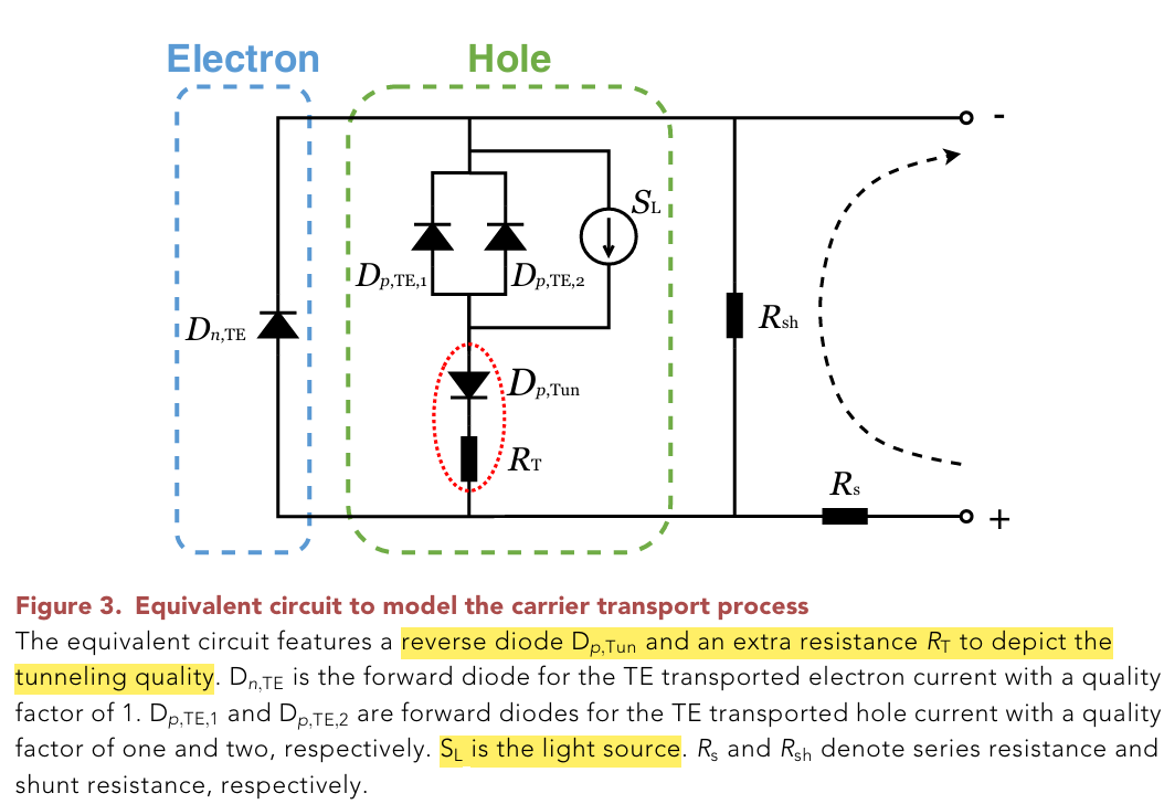
SHJ，DFHJ(dopant-free heterojunctions)电池，薄膜硅电池以及钙钛矿太阳能电池有时会存在具有S型特征的IV曲线（the S-type character of the I-V curve），即IV曲线在最大功率点的地方发生弯曲，而且暗电流和光生电流的IV曲线存在差异（discrepancies），传统的单二极管电阻和多二极管电阻的等效模型无法体现。作者对SHJ电池相关的隧穿复合模型进行考虑（$D_{p,TE,1}$，$R_T$），改进了多二极管电阻等效模型（7参数等效模型）。
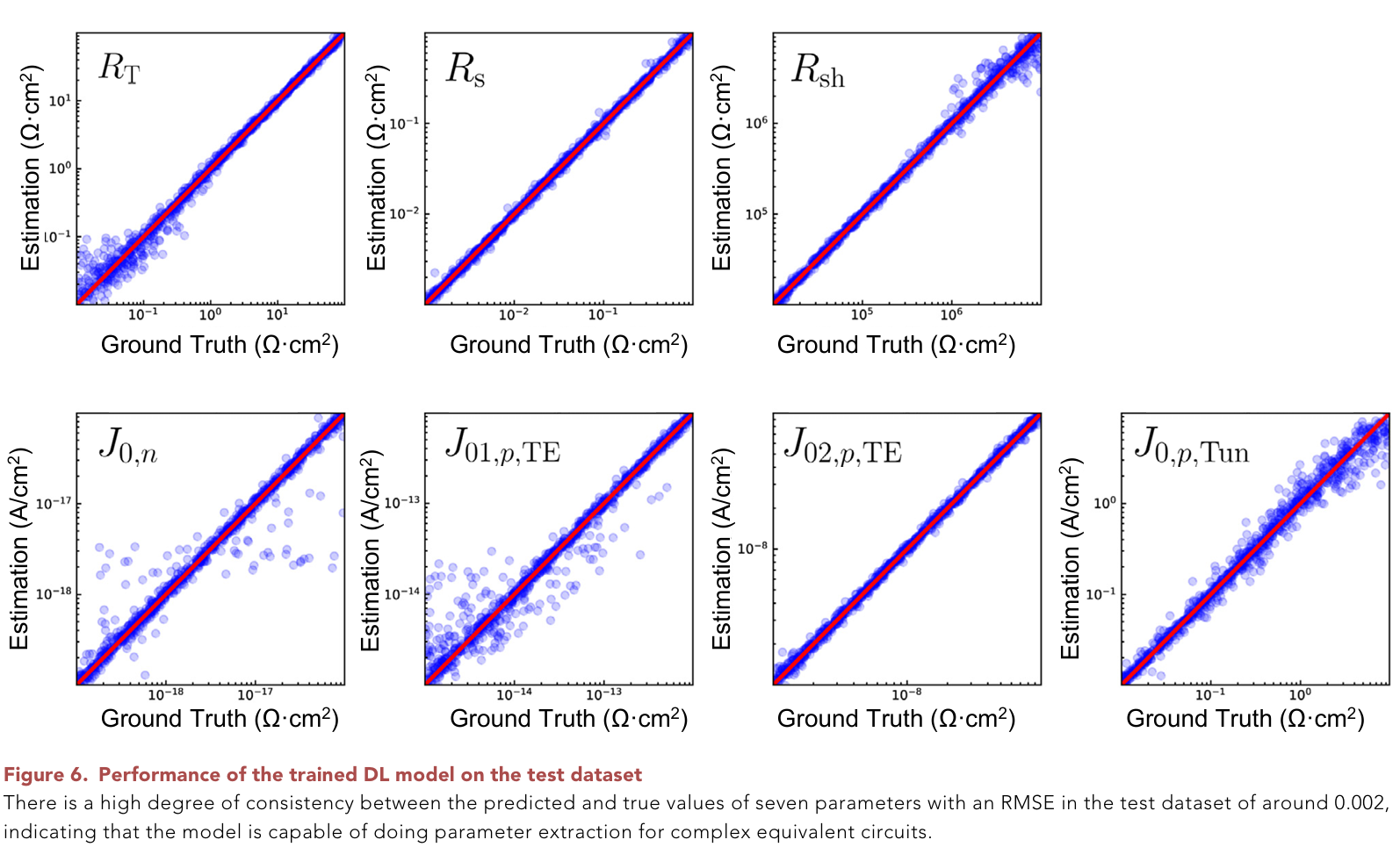
求解二极管电阻模型参数的方法通常是外推法（extrapolation method）或直接求解，但这种方法还是较为费时，作者设计了一种1d-conv+MLPs的混合模型，选择实验数据和计算数据建立数据集，以iv曲线上数据点为输入，八参数为预测输出。有较好的回归精度（有些表现不算好，但计算出iv曲线效果很好）

具体内容：

1.选择一种DFSJ电池模型（图1）造了一个样品

对样品进行不同温度的退火实验，获取了不同退火温度下的S型畸变IV曲线（图2）。作者提出高温退火导致电池后部的氧化层界面势垒增高，阻止载流子传输。

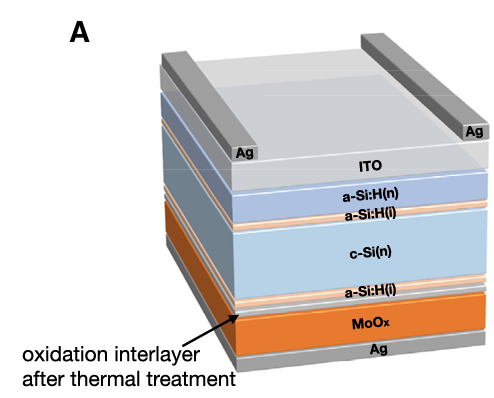
图1：DFSJ电池结构

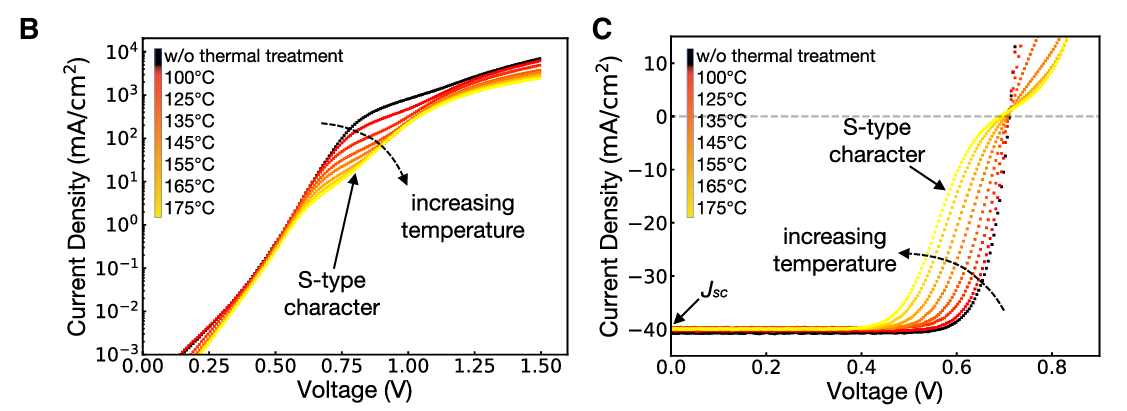
图2：B是暗电流图像，C是光生IV

Q.为什么要做高温退火:

A.多温度阶梯退火对有机聚合物太阳能电池器件性能的影响

热退火处理是本体异质结、有机聚合物太阳能电池的制备过程中非常关键的一道工序. 目前普遍认同经过热退火可以显著改善活性层的形貌[7], 优化器件的性能.在高温退火的条件下, 可以促进相分离网络中的晶化[7], 以提高器件中电荷向电极的传输能力, 从而可提高器件的效率[8].

2.作者在TCAD软件中建模，引入多种隧穿模型来仿真这一现象

模型设置：

（1）在$MoO_x$层设置trap-assisted tunneling (TAT)，陷阱辅助载流子捕获或发射

（2）界面能带尖峰设置direct tunneling (DT)

（3）导带和价带间的带带隧穿band-to band tunneling (BTBT)

（4）载流子弛豫发射过程 thermionic emission (TE)，可以等效成一个二极管（高能量时可以通过，但低能级时是无法自发到高能级上的，类似二极管的单向导通性）

hTE的二极管示意图是不是有问题呢？

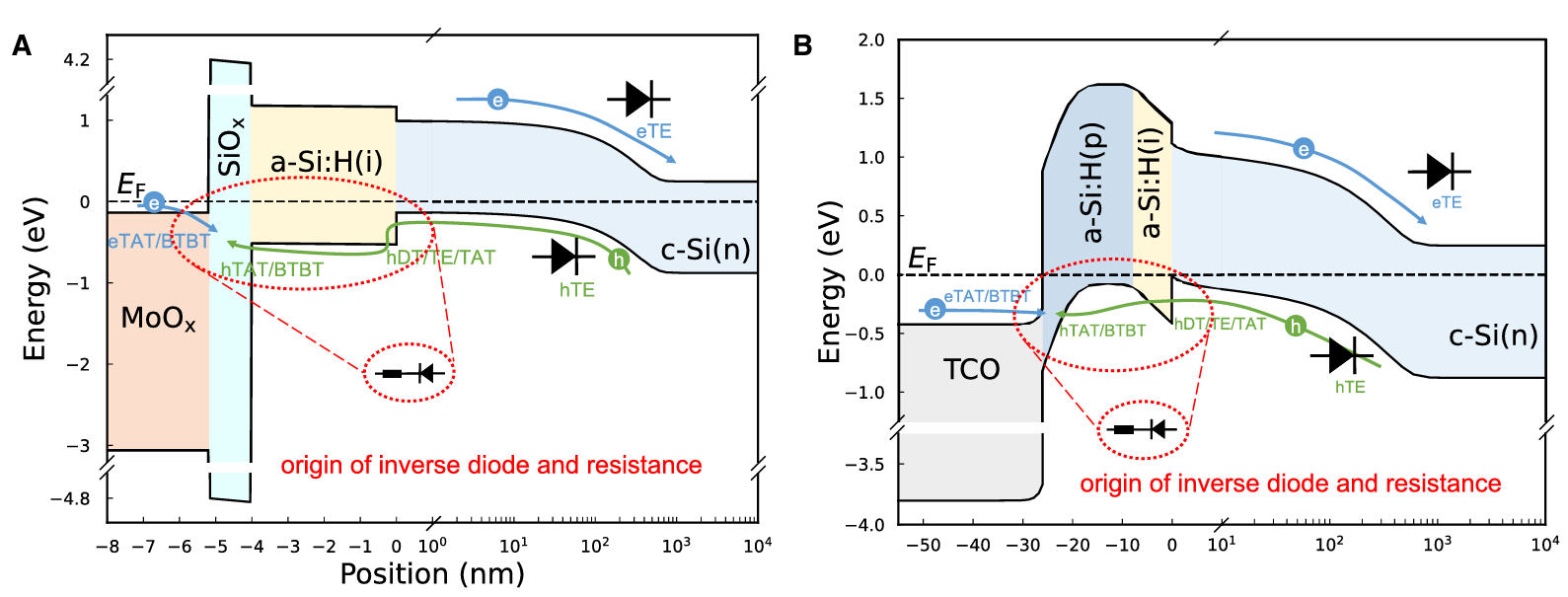
图3：A.DFSJ能带 B.SHJ能带

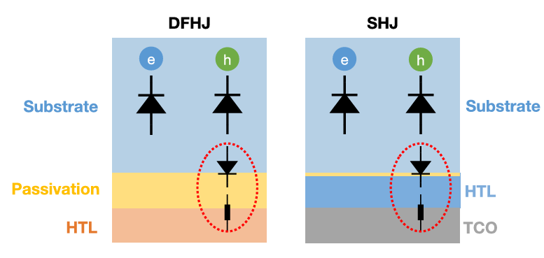
图4：模型示例（二极管代表单向导通性，电阻代表隧穿质量）

氧化硅厚度和氧化钼的掺杂，功函数影响隧穿质量，进而导致S曲线

In addition, tunneling across the MoOx=a-Si:H(i) interface should also be efficient, which is influenced by the work function of MoOx, the distribution of traps for TAT, and the barrier introduced by the oxidation interlayer.

3.引入等效电路模型：

等效电路可由equation 1.描述，J是输出电流：

$V_{th}=kT/q$，为热电压，q, k,andT are the elementary charge con stant, Boltzmann constant, and temperature

反向隧穿结的电压$V_{p,Tun}$用equation 2限制

以上7个参数对S型曲线的不同影响：

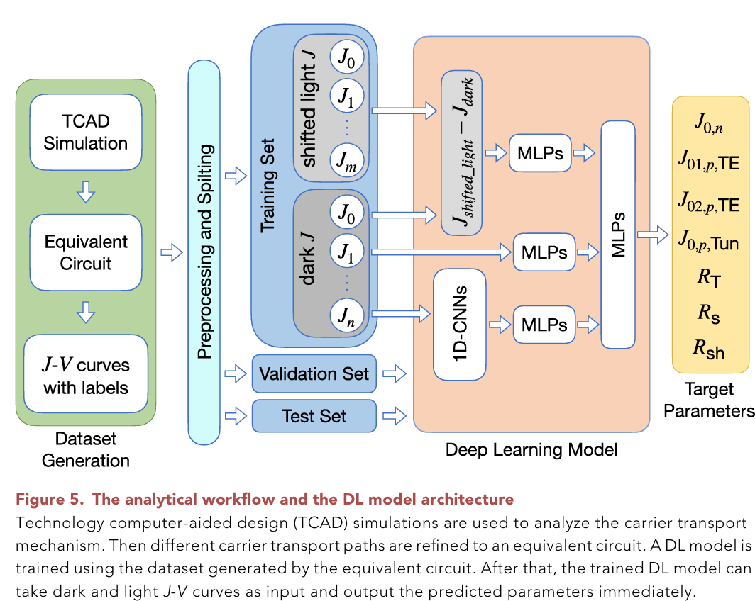
4.建立深度学习模型，直接预测对应的7参数数值：

建立数据集：

数据集构成：7列标签，51列暗电流，51列光生电流，实验数据＋Python随机生成数据

搭建网络结构：

结构图如下。

三个网络，网络1：暗电流先通过1d-conv提取特征，送入mlp训练

网络2：暗电流直接送入mlp，这是原始特征网络

网络3：光生电流与暗电流作差，求出位移量，送入mlp训练

三个网络的结果最后做concat，再送入1层mlp，降维到7个输出结果

talk is cheap, 看相关代码吧：

# combine dark and light   
class Net7(nn.Module):
  
    def __init__(self):
        super(Net7, self).__init__()
        self.cv_a1 = nn.Conv1d(1,2,5,padding=2)  # in-channel,  out-channel,  kernel-size
        self.nm_a1 = nn.LayerNorm([2,51])
        self.cv_a2 = nn.Conv1d(2,2,5,padding=2)
        self.nm_a2 = nn.LayerNorm([2,51])
        self.fc_a1 = nn.Linear(51*2,128)
        self.nm_a3 = nn.LayerNorm(128)
        self.fc_a2 = nn.Linear(128,64)
        self.nm_a4 = nn.LayerNorm(64)
        self.fc_a3 = nn.Linear(64,32)
        self.nm_a5 = nn.LayerNorm(32)
        self.fc_a4 = nn.Linear(32,7)
  
        self.fc_b1 = nn.Linear(51,128)
        self.nm_b1 = nn.LayerNorm(128)
        self.fc_b2 = nn.Linear(128,64)
        self.nm_b2 = nn.LayerNorm(64)
        self.fc_b3 = nn.Linear(64,32)
        self.nm_b3 = nn.LayerNorm(32)
        self.fc_b4 = nn.Linear(32,7)
  
        self.cv_c1 = nn.Conv1d(1,2,5,padding=2)  # in-channel,  out-channel,  kernel-size 
        self.nm_c1 = nn.LayerNorm([2,36])
        self.cv_c2 = nn.Conv1d(2,2,5,padding=2)
        self.nm_c2 = nn.LayerNorm([2,36])
        self.fc_c1 = nn.Linear(36*2,128)
        self.nm_c3 = nn.LayerNorm(128)
        self.fc_c2 = nn.Linear(128,64)
        self.nm_c4 = nn.LayerNorm(64)
        self.fc_c3 = nn.Linear(64,32)
        self.nm_c5 = nn.LayerNorm(32)
        self.fc_c4 = nn.Linear(32,7)
  
        self.fc_d1 = nn.Linear(36,64)
        self.nm_d1 = nn.LayerNorm(64)
        self.fc_d2 = nn.Linear(64,32)
        self.nm_d2 = nn.LayerNorm(32)
        self.fc_d3 = nn.Linear(32,1)
  
        self.fc = nn.Linear(7*2+1,7)
  
    def forward(self, x1, x2):
        a = F.relu(self.nm_a1(self.cv_a1(x1)))
        a = F.relu(self.nm_a2(self.cv_a2(a)))
        a = a.view(a.shape[0],-1)  # torch.flatten(x, 1), flatten all dimensions except the batch dimension
        a = F.relu(self.nm_a3(self.fc_a1(a)))
        a = F.relu(self.nm_a4(self.fc_a2(a)))
        a = F.relu(self.nm_a5(self.fc_a3(a)))
        a = self.fc_a4(a)
  
        b = x1.view(x1.shape[0],-1)
        b = F.relu(self.nm_b1(self.fc_b1(b)))
        b = F.relu(self.nm_b2(self.fc_b2(b)))
        b = F.relu(self.nm_b3(self.fc_b3(b)))
        b = self.fc_b4(b)
  
        # c = F.relu(self.nm_c1(self.cv_c1(x2)))
        # c = F.relu(self.nm_c2(self.cv_c2(c)))
        # c = c.view(c.shape[0],-1)  # torch.flatten(x, 1), flatten all dimensions except the batch dimension
        # c = F.relu(self.nm_c3(self.fc_c1(c)))
        # c = F.relu(self.nm_c4(self.fc_a2(c)))
        # c = F.relu(self.nm_c5(self.fc_a3(c)))
        # c = self.fc_c4(c)
  
        d = x2.view(x2.shape[0],-1) - x1.view(x1.shape[0],-1)[:,-36:]
        d = F.relu(self.nm_d1(self.fc_d1(d)))
        d = F.relu(self.nm_d2(self.fc_d2(d)))
        d = self.fc_d3(d)
  
  
        x = self.fc(torch.cat((a,b,d),dim=1))
  
        return x

预测结果：测试集上平均RMSE 0.002，但部分参数回归精度感觉不算好

实际iv曲线预测效果，从图上看起来还可以：

感觉可以改进的创新点：

1.知道s型曲线的模型了，能拿来做些什么事呢？

2.深度学习网络结构可以改进：

用1d-conv的目的无非就是提取参数，但1d-conv表现不是最好的，换成transformer结构呢？

self-attention block可以提取数据之间以及数据本身的信息

残差块结构可以保留原始数据特征，就不用额外的mlp结构了